Spatial Analysis of Positive and Negative tweets

Finally we conducted spatial analysis of positive and negative emotions by calculating their spatial autocorrelations with Pysal for tweets across US.

Build spatial weight matrix

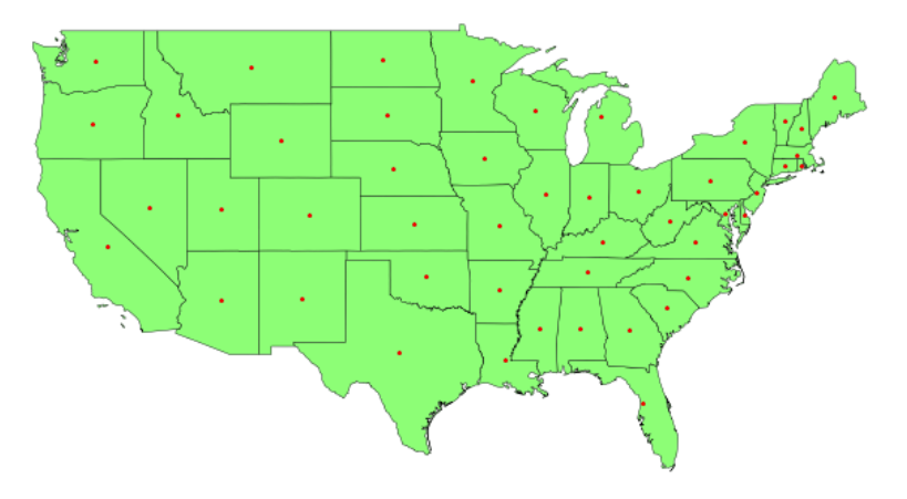
Spatial weight matrix is first built by finding the 5 nearest neighbours (here k=5).

us_centroid = merged_emo[['geometry']].copy()
us_centroid.geometry = merged_emo.centroid
fig, ax = plt.subplots(1, figsize=(11,8.5))
ax.axis('off')
us_centroid.plot(ax=ax, marker='*', color='red', markersize=1)
merged_emo.plot(ax=ax, facecolor="none", linewidth=0.4, edgecolor='0')

#k-nearest neighbour
swm5 = KNN.from_dataframe(merged_emo, k=5)

the Global Moran’s I

The Spatial Autocorrelation tool measures spatial autocorrelation based on both feature locations and feature values simultaneously. Given a set of features and an associated attribute, it evaluates whether the pattern expressed is clustered, dispersed, or random. The tool calculates the Moran’s I Index value and both a a z-score and p-value to evaluate the significance of that Index. P-values are numerical approximations of the area under the curve for a known distribution, limited by the test statistic.
The Global Moran’s I for both positive and negative tweets are around 0.2, with P-value smaller than 0.05. This suggests that the spatial autocorrelation of both positive and negative tweets is week at global scale.

pos_mi = Moran(merged_emo.positive, swm5)
print("Global Moran's I for positive tweets:", pos_mi.I) 
print("Global Moran's p-value: %0.19f" % pos_mi.p_norm)

Global Moran’s I for positive tweets: 0.20532576507819358
Global Moran’s p-value: 0.0050474715951336346

neg_mi = Moran(merged_emo.negative, swm5)
print("Global Moran's I for negative tweets:", neg_mi.I) 
print("Global Moran's p-value: %0.19f" % neg_mi.p_norm) 

Global Moran’s I for negative tweets: 0.1751399589405492 Global Moran’s p-value: 0.0150793448129815655

Local Moran’s I

The Local Moran’s Maps in Spatial Analysis of Positive and Negative tweets are plotted, where both positive (upper) and negative (lower) tweets behave strong spatial autocorrelation in the east coast, while in the west this relationship is week.

gol = pysal.explore.esda.G_Local(merged_emo['positive'], swm5, transform='B')
merged_emo['positive_I'] = gol.Zs
cols = ["positive_I", "State_Name", "positive", "geometry"]
pos_moran=merged_emo.hvplot(c="positive_I", 
                    width=600,
                  height=350,
                    cmap='cet_CET_D9',
                    hover_cols=["positive","State_Name"])

• See the spatial analysis for the code that produced these plots.